Single transmit excitation (sTx)
Single transmit excitation (sTx)
# Import all python libraries and functions used in this notebook
import matplotlib.pyplot as plt
import numpy as np
import scipy.ndimage as skymage

from functions import simulate_b1_maps
from scipy.stats import variation
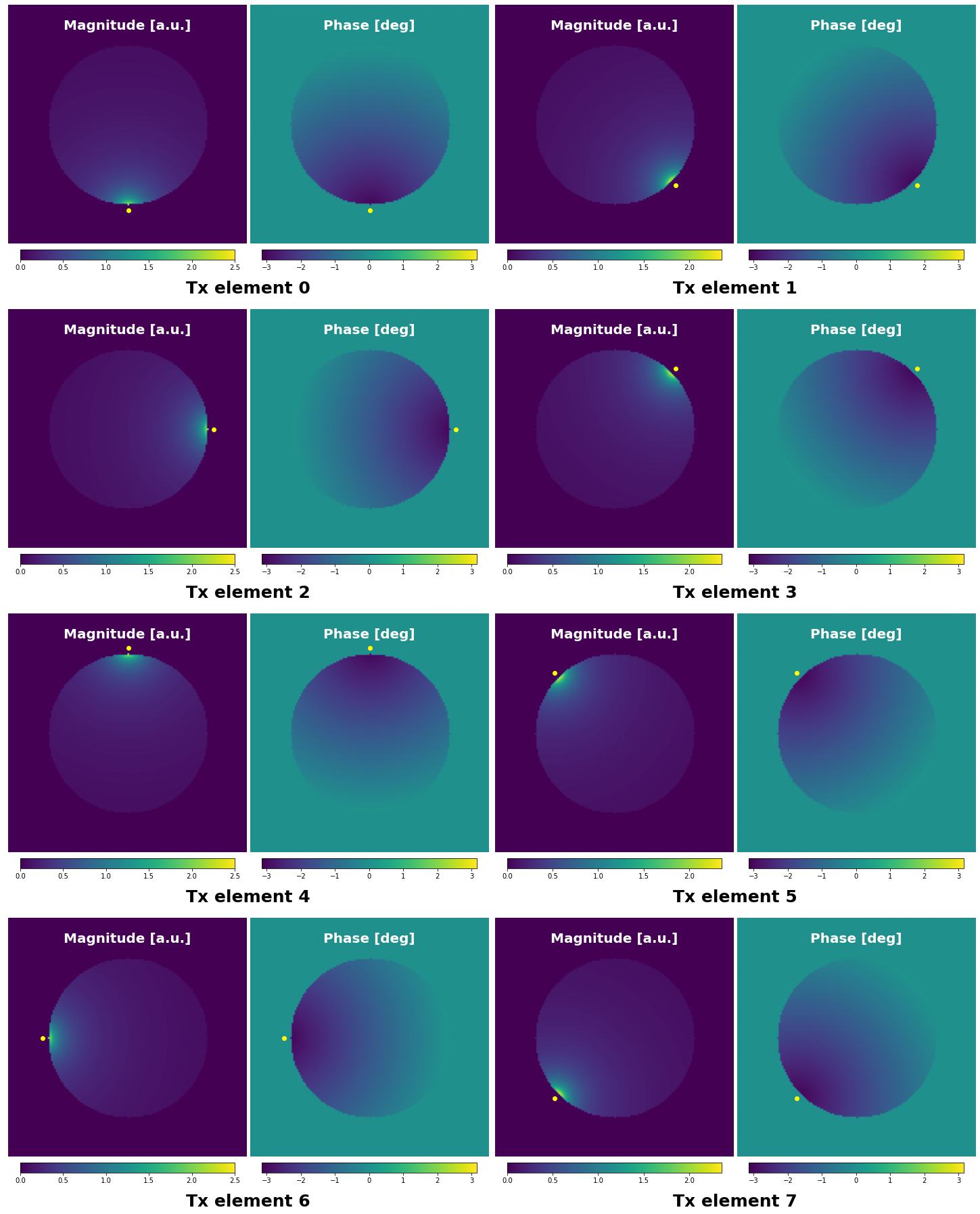
In order the produce the \(B_1^+\) field, transmit (Tx) electro-magnetic elements such as loop-coils or dipoles are excited with an current waveform. In order to produce a \(B_1^+\) field that efficiently tilts the spins out of their equilibrium position, the simpliest waveform is a sinusoidal wave at the Larmor frequency.
As discussed in the introduction, the \(B_1^+\) wavelength for low-field MRI application is larger than most body dimensions. This means that, even if the Tx elements are located far from the imaged region (e.g. outside of the bore), low field scanners can excite all transmit elements with the same waveform and produce a fairly homogeneous \(B_1^+\) field, because the dephasing between de different transmit elements will be small, and constructive RF interferences will occur.
In the early decades of MRI, scanners thus only had a single current channel used to excite all the Tx elements simulteneously with a unique waveform. This is referred to as a single transmit (sTx) system.
In the simplified example below, a 100px diameter sphere is simulated, and 8 transmit elements (yellow dots) evenly placed around it are simultaneously excited emitting a \(B_1^+\) field with a wavelength of 200px, resulting in slow phase variations.
n_Tx = 8 # Number of transmit elements to simulate
b1_maps, Tx_positions = simulate_b1_maps(n_Tx, 200)  # We simulate a RF excitation with a 200px wavelentgh
magnitude = np.abs(b1_maps)
phase =np.angle(b1_maps)

fig = plt.figure(figsize = [20, 25])
fig.subplots_adjust(wspace=0, hspace=0)
subfigs = fig.subfigures(n_Tx//2, 2, wspace=0, hspace=0)

for n, subfig in enumerate(subfigs.flat):
    subfig.suptitle(f'Tx element {n}', y=0.05, fontsize=25, weight='bold')
    axs = subfig.subplots(1, 2)
    axs[0].set_title('Magnitude [a.u.]', fontsize=20, y=0.88, color='white', weight='bold')
    axs[0].plot(Tx_positions[n, 1], Tx_positions[n, 0], 'o', color=(1, 1, 0))
    im_mag = axs[0].imshow(magnitude[:,:,n])
    plt.colorbar(im_mag, ax=axs[0], shrink=0.9, pad=0.02, orientation='horizontal')
    axs[0].axis('off')
    axs[1].set_title('Phase [deg]', fontsize=20, y=0.88, color='white', weight='bold');
    im_phase = axs[1].imshow(phase[:,:,n], vmin=-np.pi, vmax=np.pi)
    axs[1].plot(Tx_positions[n, 1], Tx_positions[n, 0], 'o', color=(1, 1, 0))
    plt.colorbar(im_phase, ax=axs[1], shrink=0.9, pad=0.02, orientation='horizontal')
    axs[1].axis('off')
plt.tight_layout(pad=1, rect=(0, 0, 1, 1))
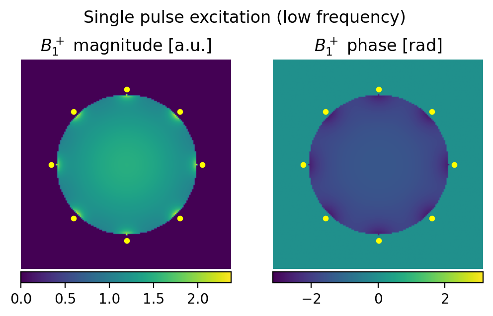
The total \(B_1^+\) field produced by a coil is the sum of all the individual complex \(B_{1n}^+\) fields produced by the \(N_{Tx}\) transmit elements of the coil.
If we assume that all transmit elements simultaneously receive the same excitation waveform (RF pulse), which is often referred to as a “single-pulse excitation”, this formula becomes:
The total \(B_1^+\) field obtained from our simulated \(B_1^+\) maps is shown below. The magnitude of the \(B_1^+\) field that will be proportional to the MR image intensity is quite homogeneous, despite some higher values close to the edges due to the proximity of the Tx elements.
b1_sTx = b1_maps @ np.ones(n_Tx)  # Complex sum corresponding to a single pulse excitation

plt.figure(dpi=200)
plt.suptitle("Single pulse excitation (low frequency)", y=0.9)
plt.subplot(121)
plt.imshow(np.abs(b1_sTx)); plt.axis('off'); plt.title("$B_1^+$ magnitude [a.u.]");
plt.colorbar(orientation="horizontal", pad=0.01)
plt.scatter(Tx_positions[:, 1], Tx_positions[:, 0], s=10, marker='o', color=(1, 1, 0))

plt.subplot(122)
plt.imshow(np.angle(b1_sTx), vmin=-np.pi, vmax=np.pi); plt.axis('off'); plt.title("$B_1^+$ phase [rad]");
plt.colorbar(orientation="horizontal", pad=0.01)

plt.scatter(Tx_positions[:, 1], Tx_positions[:, 0], s=10, marker='o', color=(1, 1, 0))
plt.show()
Now, let see what happens when the wavelength of the \(B_1^+\) field is smaller than the sphere diameter, as it is the case with Ultra-High-Field applications that require high frequency RF pulses.
b1_maps_small_wavelength, Tx_positions = simulate_b1_maps(n_Tx, wavelength_size=90)  # The wavelength size is now 90 pixel
magnitude_small_wavelength = np.abs(b1_maps_small_wavelength)
phase_small_wavelength = np.angle(b1_maps_small_wavelength)

fig = plt.figure(figsize = [20, 25])
fig.subplots_adjust(wspace=0, hspace=0)
subfigs = fig.subfigures(n_Tx//2, 2, wspace=0, hspace=0)

for n, subfig in enumerate(subfigs.flat):
    subfig.suptitle(f'Tx element {n}', y=0.05, fontsize=25, weight='bold')
    axs = subfig.subplots(1, 2)
    axs[0].set_title('Magnitude [a.u.]', fontsize=20, y=0.88, color='white', weight='bold')
    axs[0].scatter(Tx_positions[n, 1], Tx_positions[n, 0], marker='o', color=(1, 1, 0))
    im_mag = axs[0].imshow(magnitude_small_wavelength[:,:,n])
    plt.colorbar(im_mag, ax=axs[0], shrink=0.9, pad=0.02, orientation='horizontal')
    axs[0].axis('off')
    axs[1].set_title('Phase [deg]', fontsize=20, y=0.88, color='white', weight='bold');
    im_phase = axs[1].imshow(phase_small_wavelength[:,:,n], vmin=-np.pi, vmax=np.pi)
    axs[1].scatter(Tx_positions[n, 1], Tx_positions[n, 0], marker='o', color=(1, 1, 0))
    plt.colorbar(im_phase, ax=axs[1], shrink=0.9, pad=0.02, orientation='horizontal')
    axs[1].axis('off')
plt.tight_layout(pad=1, rect=(0, 0, 1, 1))
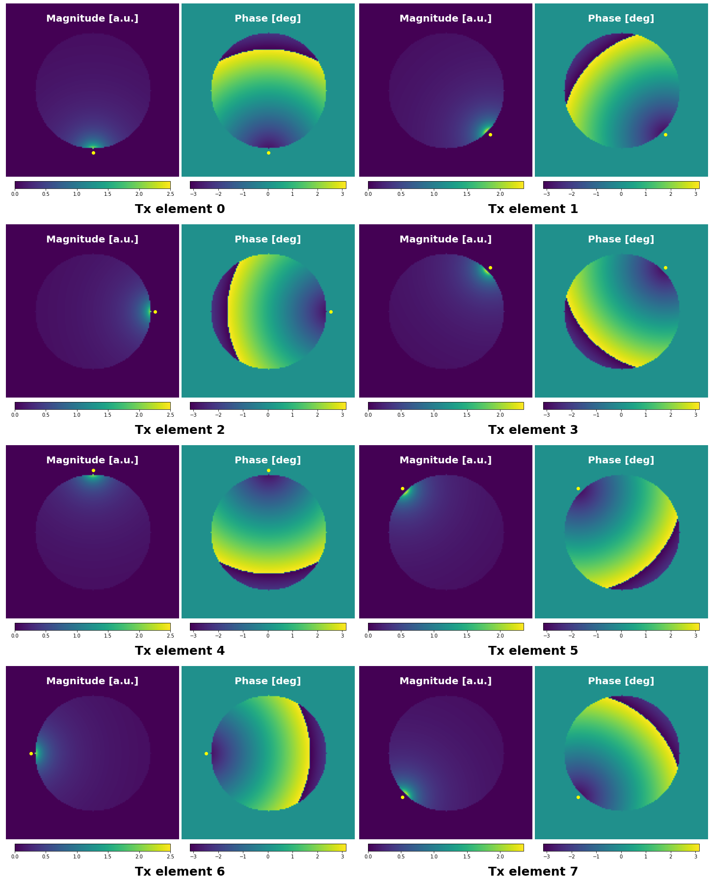
We now observe a rapid phase variation across the sphere that will modify the RF interferences pattern between the Tx elements. The high transition (yellow to dark blue) corresponds to a phase wrapping (\(-pi\) to \(pi\)). Let’s see how the summed \(B_1^+\) across elements now looks like at the higher frequency range:
b1_sTx_small_wavelength = b1_maps_small_wavelength @ np.ones(n_Tx)

plt.figure(dpi=200)
plt.suptitle("Single pulse excitation (high frequency)", y=0.9)

plt.subplot(121)
plt.imshow(np.abs(b1_sTx_small_wavelength)); plt.axis('off'); plt.title("$B_1^+$ magnitude");
plt.colorbar(orientation="horizontal", pad=0.01)
plt.scatter(Tx_positions[:, 1], Tx_positions[:, 0], s=10, marker='o', color=(1, 1, 0))

plt.subplot(122)
plt.imshow(np.angle(b1_sTx_small_wavelength), vmin=-np.pi, vmax=np.pi); plt.axis('off'); plt.title("$B_1^+$ phase");
plt.colorbar(orientation="horizontal", pad=0.01)
plt.scatter(Tx_positions[:, 1], Tx_positions[:, 0], s=10, marker='o', color=(1, 1, 0))
plt.show()
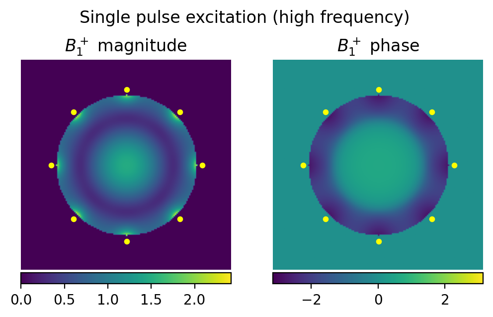
We now observe less homogeneity of the \(B_1^+\) distribution across the imaged region, which will inevitably result in an inhomogeneous image intensity and contrast (due to the inhomogeneous variable flip angle). A typical signature of \(B_1^+\) profile at UHF is the bright signal in the middle of the sphere. This phenomenon also occurs during actual head imaging and is commonly referred to as “central brightening”.