Circular polarization (CP mode)
Contents
Circular polarization (CP mode)
# Import all python libraries and functions used in this notebook
import matplotlib.pyplot as plt
import numpy as np
import scipy.ndimage as skymage

from functions import simulate_b1_maps, print_cov
from scipy.stats import variation
To reduce the \(B_1^+\) inhomogeneities that we saw in the previous chapter, we could modify the phase of the pulse that is sent by each individual Tx element to achieve a phase coherence when summing the RF signal sent by all Tx in the region of interest. This would result in less destructive RF interferences and a more homogeneous \(B_1^+\) field. This method is analogous to the phased-array method to boost the detection in radar applications, but here we use the same principle for transmission. When there are multiple Tx elements distributed around the region of interest, we want those Tx elements to produce a constructive RF excitation profile simultaneously, that is, the phase of the pulse sent by each Tx element depends on the spatial location of that element. For example, if two Tx elements are positioned at a 90° angle, then the first one will send a pulse with a 0 degree phase while the second will send the pulse with a \(pi/2\) delay. If we now place a 3rd Tx element opposite to the first element, it would send the pulse with a \(pi\) phase delay.
This type of excitation is called circular polarization (CP). As its names implies, it consists of generating a circularly polarized RF field by exciting Tx elements evenly spaced all around the subject with regularly spaced phases from 0 to 2\(\pi\). CP excitation can be achieved on a single transmit (sTx) system by using phase shifter circuits on the wiring of the different Tx elements. The inconvenience of an sTx system is that the phase is fixed for each element, which gives no freedom to modify the phase in case the excitation profile needs to be slightly modified. Conversely, parallel transmit (pTx) systems are specifically designed to send a pulse with a desired shape, magnitude and phase on each of the available channels. There could be 2, 8, 16 or even more pTx channels depending on the system. Obviously, more channels come at higher price.
Note
CP mode is efficient when used with classic circular volume coils with evenly spaced Tx elements such as birdcage or TEM coils, but it is not necessarily compatible with more complicated coil designs that are becoming increasingly popular. In these cases, the coil manufacturer will usually provide a set of phase values to use as a default excitation mode and might sometimes be referred to as “CP mode”, even if it does not exactly do a true circular polarization.
Using the same simulated \(B_1^+\) field as in the previous section, let’s compare the single pulse excitation (i.e., same phase everywhere) with the CP mode:
n_Tx = 8 # Number of transmit elements to simulate
b1_maps, Tx_positions = simulate_b1_maps(n_Tx, 90)

b1_sTx = b1_maps @ np.ones(n_Tx)  # Single pulse excitation
b1_CP = b1_maps @ np.exp(1j * np.linspace(0, 2*(np.pi - np.pi / n_Tx), n_Tx))  # CP mode

plt.figure(figsize=(17, 14), constrained_layout=True)
plt.suptitle("Single pulse excitation vs CP mode", fontsize=30, y=1.05)
plt.subplot(221)
plt.imshow(np.abs(b1_sTx)); plt.axis('off'); plt.title("Single pulse excitation", fontsize=25);
plt.text(54, 12, "Magnitude [u.a.]", color='white', fontsize=25)
plt.clim([0, 3])
plt.colorbar(pad=0.01)
plt.scatter(Tx_positions[:, 1], Tx_positions[:, 0], s=50, marker='o', color=(1, 1, 0))
plt.subplot(222)
plt.imshow(np.abs(b1_CP)); plt.axis('off'); plt.title("CP mode", fontsize=25);
plt.text(54, 12, "Magnitude [u.a.]", color='white', fontsize=25)
plt.clim([0, 3])
plt.colorbar(pad=0.01)
plt.scatter(Tx_positions[:, 1], Tx_positions[:, 0], s=50, marker='o', color=(1, 1, 0))
plt.subplot(223)
plt.imshow(np.angle(b1_sTx), vmin=-np.pi, vmax=np.pi); plt.axis('off');
plt.text(64, 12, "Phase [rad]", color='white', fontsize=25)
plt.colorbar(pad=0.01)
plt.scatter(Tx_positions[:, 1], Tx_positions[:, 0], s=50, marker='o', color=(1, 1, 0))
plt.subplot(224)
plt.imshow(np.angle(b1_CP)); plt.axis('off');
plt.text(64, 12, "Phase [rad]", color='white', fontsize=25)
plt.colorbar(pad=0.01)
plt.scatter(Tx_positions[:, 1], Tx_positions[:, 0], s=50, marker='o', color=(1, 1, 0))
plt.show()
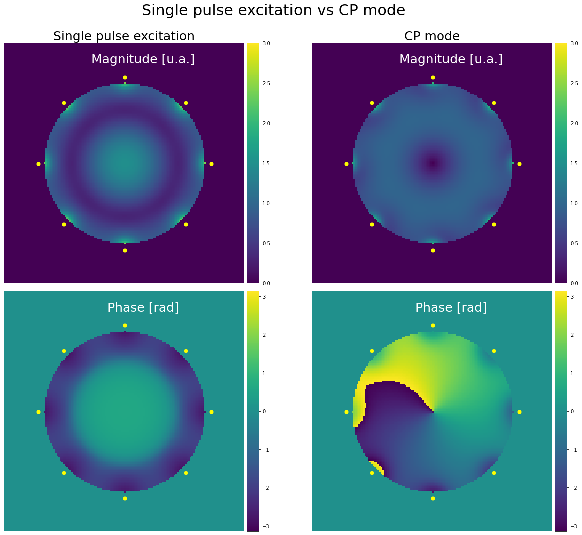
The CP mode results in a more homogeneous magnitude profile and helps getting rid of the central brightening effect. However, it results in a very low \(B_1^+\) in the middle of the sphere, which could be problematic from an imaging standpoint.
The phase images illustrate particularly well the circular aspect of the polarization.
In order to evaluate the benefits of the CP mode regarding the \(B_1^+\) homogeneity, we need to quantify the homogeneity obtained with both scenarios. A useful metric to do so is the coefficient of variation (CoV or CV) which is defined as the standard deviation of the total \(B_1^+\) field divided by its mean value:
From the formula above, we understand that a homogeneous \(B_1^+\) field is associated with a low CoV.
In our simulation, we get the following CoV values:
print(f"CoV (single pulse): {variation(np.abs(b1_sTx[b1_sTx!=0])):.3f}")  # CoV in the mask - single pulse
print(f"CoV (CP mode): {variation(np.abs(b1_CP[b1_CP!=0])):.3f}")  # CoV in the mask - CP mode
print(f"{variation(np.abs(b1_sTx[b1_sTx!=0]))/variation(np.abs(b1_CP[b1_CP!=0])):.2f} fold CoV decrease")  # Ratio
CoV (single pulse): 0.465
CoV (CP mode): 0.196
2.37 fold CoV decrease
These results show that, in this particular example, the CP mode is very efficient at homogenizing the \(B_1^+\) field as it results in a 2.37 lower CoV compared to a single pulse excitation. However, these benefits clearly depend on the geometry of the subject, the position of the transmit elements and the RF wavelength.
Effect of the wavelength on the CP mode benefits
To better assess how the RF wavelength impacts the homogeneity improvement of the CP mode compared to single pulse in a given coil configuration, let’s run the previous simulation while varying the RF wavelength and return the CoV ratio corresponding to each wavelength:
phases = np.linspace(0, 2*(np.pi-np.pi/n_Tx), n_Tx)
weights_sTx = np.ones(n_Tx)/np.sqrt(n_Tx)
weights_CP = np.ones(n_Tx) / np.sqrt(n_Tx) * np.exp(1j * phases)

wavelength_values = np.linspace(1, 150, 50)  # Array of wavelengths to test
CoV_ratio = []
for n, wavelength in enumerate(wavelength_values):

    b1_maps, _ = simulate_b1_maps(n_Tx, wavelength)

    b1_sTx = b1_maps @ weights_sTx
    b1_CP = b1_maps @ weights_CP

    CoV_ratio.append(variation(np.abs(b1_sTx[b1_sTx!=0]))/variation(np.abs(b1_CP[b1_CP!=0])))

plt.figure(figsize=(17, 6))
plt.plot(wavelength_values, CoV_ratio, linewidth=3)
plt.title("Benefits of CP mode against single pulse", fontsize=25, pad=20)
plt.xlabel("Wavelength in % of sphere diameter", fontsize=20, labelpad=20)
plt.ylabel("CoV(sTx) / CoV(CP)", fontsize=20, labelpad=20)
plt.tick_params(axis='both', labelsize=15)
plt.show()
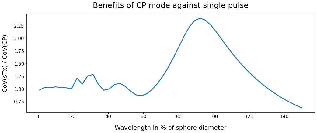
This graph shows that, in this coil configuration, the best CP mode is obtained when the excitation frequency is about 90% of the sphere diameter.
However in “real world” MRI, the required RF frequency depends on the magnet’s nominal \(B_0\) strength and the type of imaged spins. For example, at 7T 1H proton imaging, the excitation frequency needs to be about 300 MHz. The RF designer this should adapt the coil geometry to get a good \(B_1^+\) homogeneity while also taking into account parameters such as the receive sensitivity of the coil, the coupling between the RF elements and the energy deposition into the subject’s tissues.