Complex B_1^+ shimming
Contents
Complex \(B_1^+\) shimming
# Import all python libraries and functions used in this notebook
import matplotlib.pyplot as plt
import numpy as np

import scipy

from functions import *
from scipy.stats import variation
Optimizing the phase and magnitude of the shim weights
In the previous section (phase-only shimming), we demonstrated how optimizing the phase of the shim weights can improve the \(B_1^+\) homogeneity. In this section we investigate what happens if we optimize both the phase and the magnitude values of the shim weights, thus adding more degrees of freedom to the optimization process.
Note
Because Scipy optimization algorithms do not handle complex variables, the shim weights phases and magnitudes are reshaped into an vector of length \(2 \times N_{Tx}\) over which the optimization is performed.
# Load the data
b1_maps = np.load('./data/b1_maps.npy')  # Complex 2D B1 maps of each element (x, y, n_coils)
x, y, n_Tx = b1_maps.shape  # Number of transmit elements
mask = b1_maps.sum(-1) != 0

# Single pulse excitation
weights_sTx = np.ones(8)
b1_sTx = (b1_maps @ weights_sTx)

# CP mode
weights_CP = np.exp(1j * np.linspace(0, 2*(np.pi - np.pi / n_Tx), n_Tx)) # CP weights
b1_CP = b1_maps @ np.exp(1j * np.linspace(0, 2*(np.pi - np.pi / n_Tx), n_Tx))

# Phase-only shimming
weights_PO = phase_only_shimming(b1_maps)
b1_PO = b1_maps @ weights_PO

initial_weights = weights_PO  # Starting from phase-only shim weights
b1_roi = np.reshape(b1_maps * mask[:, :, np.newaxis], [b1_maps.shape[0] * b1_maps.shape[1], 8])
b1_roi = b1_roi[b1_roi[:, 0] != 0, :]

def cost_function(weights):
    return variation(np.abs(b1_roi @ vector_to_complex(weights)))

weights_PM = vector_to_complex(scipy.optimize.minimize(cost_function, complex_to_vector(initial_weights)).x)

b1_PM = np.abs(b1_maps @ weights_PM)

fig, axes = plt.subplots(1, 3, figsize=[20, 7])
vmax= np.max(np.abs(np.concatenate((b1_CP, b1_PO, b1_PM))))

axes[0].imshow(np.abs(b1_CP), vmax=vmax); axes[0].axis('off')
axes[0].set_title(f"$|B_1^+|$ (CP mode)\nCoV = {variation(np.abs(b1_CP[mask])):.2f}", fontsize=20)

axes[1].imshow(np.abs(b1_PO), vmax=vmax); axes[1].axis('off')
axes[1].set_title(f"$|B_1^+|$ (phase-only)\nCoV = {variation(np.abs(b1_PO[mask])):.2f}", fontsize=20)

im = axes[2].imshow(np.abs(b1_PM), vmax=vmax); plt.axis('off')
axes[2].set_title(f"$|B_1^+|$ (phase + magnitude)\nCoV = {variation(np.abs(b1_PM[mask])):.2f}", fontsize=20)

cbar = fig.colorbar(im, ax=axes.ravel().tolist(), shrink=0.72, pad=0.015)
cbar.ax.set_title('nT/V', fontsize=20, pad=10)
cbar.ax.tick_params(labelsize=20)

plt.show()
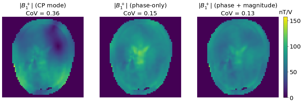
We observe that by optimizing both the phase and the magnitude of the excitation pulses, we obtain a lower CoV than in the “phase-only” case. This method is usually referred to as Static \(B_1^+\) shimming (or Static RF shimming ).
Note
Once again, this process might result in sub-optimal solutions if initial optimization values are not wisely chosen. There are even more local minima here due to the higher number of degrees of freedom.
In the example above, the complex optimization uses the phase-only shim weights as a starting point to make sure that the final \(B_1^+\) homogeneity is improved compared to the phase-only shimming scenario.
plt.figure(figsize=[17, 8])
plt.suptitle("Complex shim weights", fontsize=30, y=1.05)
plt.subplot(131)
show_weights(weights_CP)
plt.title("CP mode", fontsize=30, pad=15)
plt.subplot(132)
show_weights(weights_PO)
plt.title("Phase-only", fontsize=30, pad=15)
plt.subplot(133)
show_weights(weights_PM)
plt.title("Magnitude + phase", fontsize=30, pad=15)
plt.show()
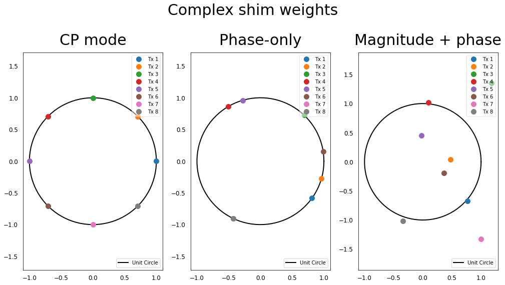
The additionnal degrees of freedom are illustrated by the fact that the shim weights are no more constrained to the unit circle but can have any magnitude value.
ROI size and local \(B_1^+\) shimming
On the previous example, we see that there might still be some local drops or hotspots of the \(B_1^+\) field after shimming. This is mainly due to the fact that there is usually no solution that yields a perfectly homogeneous \(B_1^+\) field, because we are limited by the number of transmit elements and their respective \(B_1^+\) distributions.
In the particular cases where we only want to image a specific region of interest (ROI) in the body (e.g. the spinal cord, the prostate), performing \(B_1^+\) shimming over this ROI usually results in better homogeneity.
However, the homogeneity outside of the ROI might be greatly affected by this solution, this method is thus particularly suited when we need a very homogeneous field in a small region but we don’t mind degrading the rest of the image.
Running \(B_1^+\) shimming over a small ROI is illustrated below:
mask_reduced = np.zeros(b1_maps[:,:,0].shape)
mask_reduced[x//2-10:x//2+10, y//2-10:y//2+10] = 1

b1_roi_reduced = np.reshape(b1_maps * mask_reduced[:, :, np.newaxis], [x * y, n_Tx])
b1_roi_reduced = b1_roi_reduced[b1_roi_reduced[:, 0] != 0, :]

def cost_function(weights):
    return variation(np.abs(b1_roi_reduced @ vector_to_complex(weights)))

weights_PM_masked = vector_to_complex(scipy.optimize.minimize(cost_function, complex_to_vector(initial_weights)).x)

b1_PM_masked = np.abs(b1_maps @ weights_PM_masked)

b1_PM_ROI = b1_PM * mask_reduced
b1_PM_ROI[b1_PM_ROI == 0] = np.nan

b1_PM_masked_ROI = b1_PM_masked * mask_reduced
b1_PM_masked_ROI[b1_PM_masked_ROI == 0] = np.nan

fig, axes = plt.subplots(1, 2, figsize=[20, 9])
vmax=np.nanmax(np.concatenate((b1_PM_ROI, b1_PM_masked_ROI)))

axes[0].imshow(b1_PM, cmap='gray')
axes[0].imshow(b1_PM_ROI, vmin=0, vmax=vmax); axes[0].axis('off')
axes[0].set_title(f"|$B_1^+$| (phase + magnitude)\nCoV in ROI: {variation(b1_PM[mask_reduced!=0]):.3f}\n"
                  f"CoV outside ROI: {variation(b1_PM[mask-mask_reduced!=0]):.3f}", fontsize=25)
axes[1].imshow(b1_PM_masked, cmap='gray')
im =axes[1].imshow(b1_PM_masked_ROI, vmin=0, vmax=vmax); axes[1].axis('off')
axes[1].set_title(f"|$B_1^+$| (reduced ROI)\nCoV in ROI: {variation(b1_PM_masked[mask_reduced!=0]):.3f}\n"
                  f"CoV outside ROI: {variation(b1_PM_masked[mask-mask_reduced!=0]):.3f}", fontsize=25)

cbar = fig.colorbar(im, ax=axes.ravel().tolist(), shrink=0.9, pad=0.02)
cbar.ax.set_title('nT/V', fontsize=20, pad=10)
cbar.ax.tick_params(labelsize=20)
plt.show()
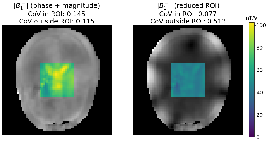
We indeed observe that \(B_1^+\) field is more homogeneous over the chosen ROI (square in the middle of the brain). As expected, the homogeneity outside of the ROI is greatly decreased as these voxels are not considered during the optimization process.
Energy deposition and SAR constraint
As we saw earlier, performing RF-shimming modifies the current sent to each transmit element and might result in RF “hotspots”. When applying an RF electromagnetic field to a patient, its electric component induces heat dissipation in the tissues, wich might be dangerous if the temperature rise becomes too important.
In order to perfom MRI scans safely, we thus limit the energy deposition in the patient. This is done by monitoring the Specific Absorbtion Rate (SAR), which corresponds to the rate at which the energy is absorbed per unit mass of tissue. This is the same metric that the one used to monitoring the RF emissions of mobile phones, and it is usually expressed in watts per kilogram (W/kg).
As of today, no perfectly accurate method has been developped in order to measure the SAR during in-vivo MR experiments. For this reason, SAR estimations are based on sophisticated modeling of the coil/body system.
In MRI, the SAR is computed globally and locally, using the following formula:
Where \(w\) is a complex vector of length \(C\) (shim weights) and \(Q\) is a matrix of size \((C\times C)\) where C is the number of transmit channels. \(Q\) is determined through EM simulations, based on each channel’s electric field distribution.
As \(Q\) does not correspond to in-vivo measurements, a safety factor is usually applied in order to safely consider the differences between the simulated and actual experiments.
Global SAR
The global SAR is the total power absorbed by the whole body divided by the weight of the whole body. It is limited to 2W/kg by the IEC standard 60601-2-33. It is usually measured by the scanner during the scan, and pulse sequences are interrupted if the limit value is exceded.
Local SAR
The local SAR aims to limit the energy deposition in small portions of the body. During the simulation process, a Q matrix will be computed for every 10g of tissues and the limit value will be larger than for global shimming (tyically 10W/kg for the head and trunk, and 20W/kg for the extremities), in order to take the existence of local SAR hotspots into account.
SAR and Ultra High Field imaging
SAR is proportional to \(\omega_0^2\), meaning that the energy deposition at 7T is ~5 times higher than at 3T. SAR constraints will thus become even more challenging at UHF in order to ensure patient’s safety. Local SAR will be particularly constraining as the arising of SAR hotspots becomes frequent due to the use of several Tx elements positioned close to the patient.
Virtual observation points
Virtual Observation Points (VOP) are matrices used to reduce the number of Q-matrices considered during the optimization process. The principle is that the Q-matrices corresponding to all the 10g tissues are gathered in different subgroups (VOP) based on their similarities. The larger the subgroup, the less VOPs will be used for optimization, thereby accelerating the optimization process.
Note
If we want a very small number of VOPs, we have to increase the subgroup size, i.e., reduce the accuracy of the SAR computation. This might result in SAR overestimations and overconstrained optimizations (sacrificing homogeneity for lower SAR).
Let’s compare the \(B_1^+\) distribution obtained whith an unconstrained vs. constrained SAR shim weight optimization:
# Virtual observation points are stored in a .npy file
vop = np.load("./data/vop.npy")

def max_SAR(weights, vop):
    # computes max local SAR
    return np.max(np.real(np.matmul(np.matmul(np.conj(weights).T, vop.T), weights)))

SAR_limit = max_SAR(weights_CP, vop)

initial_weights = complex_to_vector(weights_PO)

b1_roi = np.reshape(b1_maps * mask[:, :, np.newaxis], [x * y, n_Tx])
b1_roi = b1_roi[b1_roi[:, 0] != 0, :]

def cost_function(weights):
    return variation(np.abs(b1_roi @ vector_to_complex(weights)))

cons = ({'type': 'ineq', 'fun': lambda x:  -max_SAR(vector_to_complex(x), vop) + SAR_limit}) # SAR constraint

weights_SAR = vector_to_complex(scipy.optimize.minimize(cost_function, initial_weights, constraints=cons).x)

b1_SAR = b1_maps @ weights_SAR

fig, axes = plt.subplots(1, 2, figsize=[20, 9])
vmax = np.abs(np.concatenate((b1_PM, b1_SAR))).max()

axes[0].imshow(np.abs(b1_PM), vmax=vmax); axes[0].axis('off')
axes[0].set_title(f"|$B_1^+$| (phase + magnitude)\nCoV in ROI: {variation(np.abs(b1_PM[mask])):.3f}\n"
          f"Mean: {np.abs(b1_PM[mask]).mean():.3f} nT/V\nMax local SAR: {SAR_limit:.3f} a.u.", fontsize=25)

im =axes[1].imshow(np.abs(b1_SAR), vmax=vmax); axes[1].axis('off')
axes[1].set_title(f"|$B_1^+$| (SAR constrained)\nCoV in ROI: {variation(np.abs(b1_SAR[mask])):.3f}\n"
          f"Mean: {np.abs(b1_SAR[mask]).mean():.3f} nT/V\nMax local SAR: {max_SAR(weights_SAR, vop):.3f} a.u.", fontsize=25)

cbar = fig.colorbar(im, ax=axes.ravel().tolist(), shrink=0.9, pad=0.02)
cbar.ax.set_title('nT/V', fontsize=20, pad=10)
cbar.ax.tick_params(labelsize=20)
plt.show()
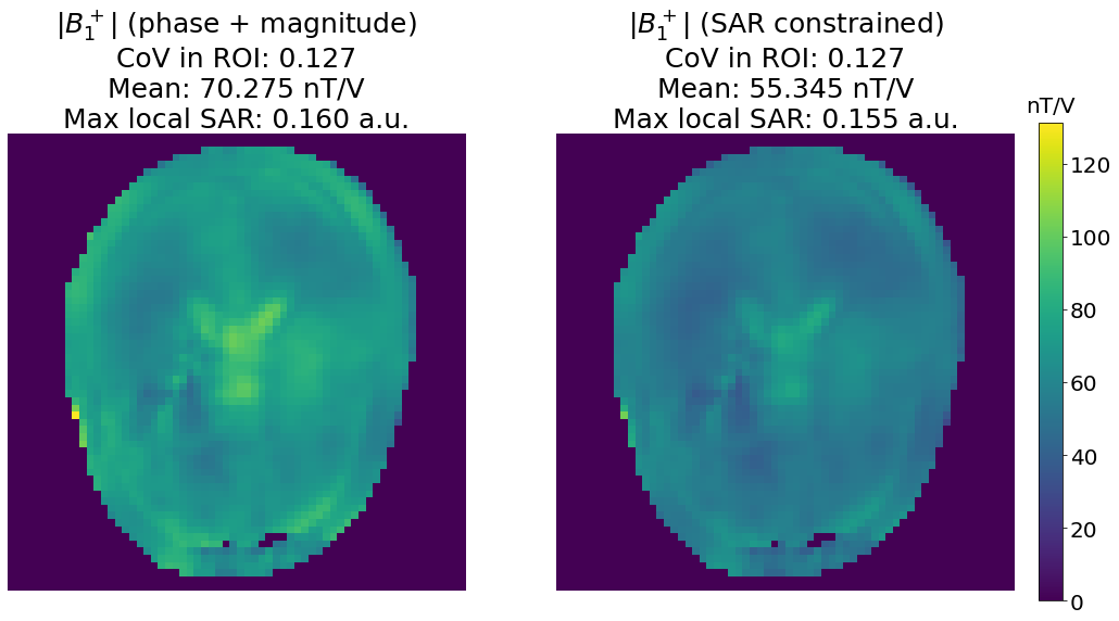
Here we managed to get the same homogeneity (as assessed by the CoV) in the SAR-unconstrained and SAR-constrained scenario. However, we observe a decrease in the mean \(B_1^+\) values, because the optimization process has reduced the shim weights magnitudes in order not to exceed the maximum local SAR of the CP mode.
Targeting a specific \(B_1^+\) value
An infinity of cost functions can be used to fulfill different goals during the optimization process.
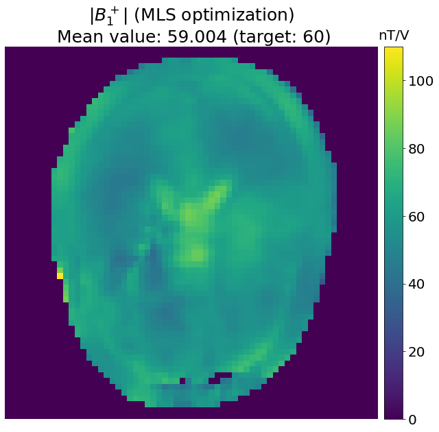
In this section, instead of trying to minimize the coefficient of variation, the goal is to minimize the difference between the combined \(B_1^+\) and a target value (here 60 nT/V) by using the following cost function:
Note
If the target value is too high to be reached without exceeding the SAR limit, the maximum reachable mean \(B_1^+\) value will be obtained, while preserving a fairly good homogeneity.
# B1+ value to target in nT/V
target = 60

def cost_function_MLS(weights):
    b1_abs = np.abs(b1_roi @ vector_to_complex(weights))
    return np.sum((b1_abs - target)**2)

weights_MLS = vector_to_complex(scipy.optimize.minimize(cost_function_MLS, initial_weights, constraints=cons).x)

b1_MLS= np.abs(b1_maps @ weights_MLS)

plt.figure(figsize=[17,10])
plt.imshow(b1_MLS); plt.axis('off')
plt.title(f"$|B_1^+|$ (MLS optimization)\n Mean value: {np.mean(b1_MLS[mask]):.3f} (target: {target})", fontsize=25)
cbar = plt.colorbar(pad=0.01)
cbar.ax.set_title('nT/V', fontsize=20, pad=10)
cbar.ax.tick_params(labelsize=20)
plt.show()
Further improving the \(B_1^+\) homogeneity
Data post processing
In order to reduce the influence of the \(B_1^+\) inhomogeneity on the final image we can perform offline image post-processing (segmentation, filtering, normalization, etc.). These methods usually require knowledge of the \(B_1+\) distribution (which can be measured or estimated from the image intensity) and cannot be used to improve the image contrast or SNR.
[1] Cohen et al. 2000. “Rapid and Effective Correction of RF Inhomogeneity for High Field Magnetic Resonance Imaging.”
[2] Wang et al. 2005. “Measurement and Correction of Transmitter and Receiver Induced Nonuniformities in Vivo.”
Pulse design
In order to get even more homogeneous \(B_1^+\) distributions, researchers have been playing with pulse design solution (sending different pulse shape on each Tx elements, depositing energy at strategic k-space locations, etc.). Pulse design is very interesting when coupled to pTx capabilities as it provides state-of-the-art \(B_1^+\) homogenizations, but this method requires extensive knowledge of the pulse design theory and is computationally demanding.
[3] Saekho et al. 2006. “Fast-Kz Three-Dimensional Tailored Radiofrequency Pulse for Reduced B1 Inhomogeneity.”
Calibration-free methods
Some homogenization methods do not require any time consuming mapping or optimization steps and are referred to as calibration-free. Among them, Universal Pulses are obtained by optimizing pulses over a set of subject to correct for the \(B_1^+\) inhomogeneities in all subsequent scanned subjects. Even if these solutions are not patient-specific, very promising results have been demonstrated in the brain, surpassing static \(B_1^+\) shimming.
[4] Gras et al. 2017. “Universal Pulses: A New Concept for Calibration‐free Parallel Transmission.”