Phase-only B_1^+ shimming
Contents
Phase-only \(B_1^+\) shimming
# Import all python libraries and functions used in this notebook
import matplotlib.pyplot as plt
import numpy as np

from functions import simulate_b1_maps, show_weights, phase_only_shimming
from scipy.stats import variation
With in-vivo \(B_1^+\) maps
The CP mode previously described is an interesting way to improve the \(B_1^+\) homogeneity, but its efficiency depends a lot on the coil geometry, the geometry of the object to image and the Larmor Frequency (which depends on the main static \(B_0\) field).
A consequence of the CP mode being dependent on the geometry of the object is that the \(B_1^+\) distribution will change across individual subjects, because every subject has a different morphometry (size, shape, tissue distribution, etc.).
To overcome this challenge, patient-specific solutions have been developped in order to take the human anatomical variability into account. These solutions consist in:
mapping the \(B_1^+\) field while the patient lies in the scanner, and then
optimizing the pulses sent to the different Tx elements in order to control the RF interferences and improve the \(B_1^+\) homogeneity.
One of the simpliest patient-specific solution in terms of hardware design and computation is the phase-only \(B_1^+\) shimming. It consists in using the in-vivo \(B_1^+\) maps to find a set of phase values that minimize the \(B_1^+\) heterogeneity, and to apply these phases to the Tx elements when scanning the patient.
Here, the shim weights are determined by minimizing the following cost function that represents the \(B_1^+\) heterogeneity:
The benefits of phase-only shimming are presented below by comparing it with the single pulse excitation and the circular polarization, using the in-vivo data introduced in the \(B_1^+\) mapping section.
# Note: This code will take a few minutes to run 😅
n_Tx = 8  # Number of transmit elements
b1_maps = np.load('./data/b1_maps.npy')  # Complex 2D B1 maps of each element (x, y, n_coils)

weights_sTx = np.ones(n_Tx)  # Single pulse weights
b1_sTx = b1_maps @ weights_sTx

weights_CP = np.exp(1j * np.linspace(0, 2*(np.pi - np.pi / n_Tx), n_Tx)) # CP weights
b1_CP = b1_maps @ np.exp(1j * np.linspace(0, 2*(np.pi - np.pi / n_Tx), n_Tx))

mask = b1_maps[:, :, 0] != 0  # 2D mask removing null values

weights_PO = phase_only_shimming(b1_maps, initial_weights=2*np.pi*np.random.rand(n_Tx))

b1_PO = b1_maps @ weights_PO  # Computing the complex phase only shimmed B1+ field

fig, axes = plt.subplots(1, 3, figsize=[20, 7])
vmax= np.max(np.abs(np.concatenate((b1_sTx, b1_CP, b1_PO))))

axes[0].imshow(np.abs(b1_sTx), vmax=vmax); axes[0].axis('off')
axes[0].set_title(f"$|B_1^+|$ (sTx)\nCoV = {variation(np.abs(b1_sTx[mask])):.2f}", fontsize=20)

axes[1].imshow(np.abs(b1_CP), vmax=vmax); axes[1].axis('off')
axes[1].set_title(f"$|B_1^+|$ (CP mode)\nCoV = {variation(np.abs(b1_CP[mask])):.2f}", fontsize=20)

im = axes[2].imshow(np.abs(b1_PO), vmax=vmax); plt.axis('off')
axes[2].set_title(f"$|B_1^+|$ (phase-only)\nCoV = {variation(np.abs(b1_PO[mask])):.2f}", fontsize=20)

cbar = fig.colorbar(im, ax=axes.ravel().tolist(), shrink=0.72, pad=0.015)
cbar.ax.set_title('nT/V', fontsize=20, pad=10)
cbar.ax.tick_params(labelsize=20)

plt.show()
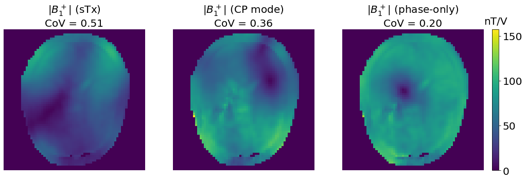
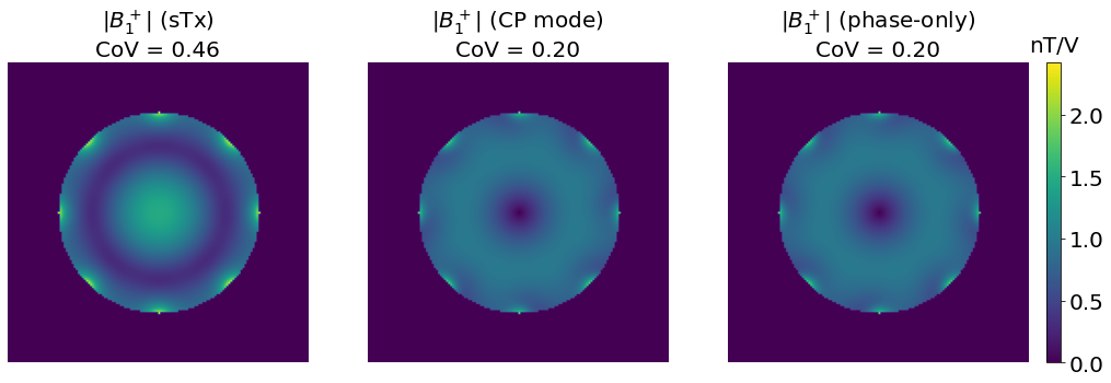
These results show a more homogeneous \(B_1^+\) profile (as assessed by the lower CoV), as well as a more efficient excitation (as assessed by the higher nT per unit voltage).
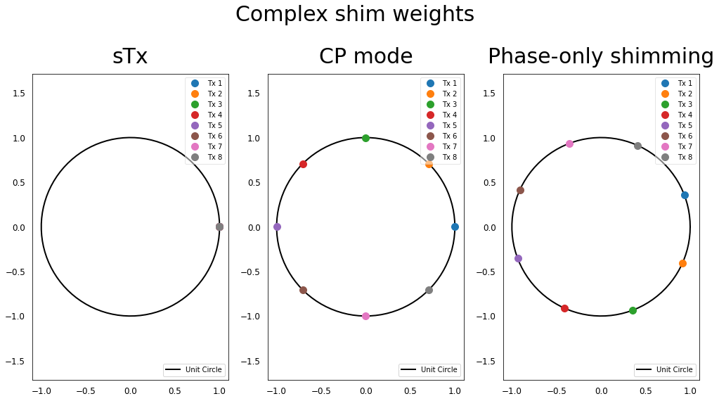
Let’s look at the complex shim weights applied on the different Tx elements for these 3 scenarios:
plt.figure(figsize=[17, 8])
plt.suptitle("Complex shim weights", fontsize=30, y=1.05)
plt.subplot(131)
show_weights(weights_sTx)
plt.title("sTx", fontsize=30, pad=15)
plt.subplot(132)
show_weights(weights_CP)
plt.title("CP mode", fontsize=30, pad=15)
plt.subplot(133)
show_weights(weights_PO)
plt.title("Phase-only shimming", fontsize=30, pad=15)
plt.show()
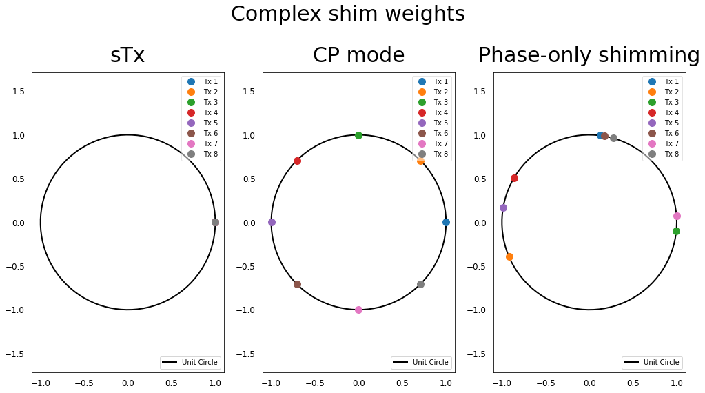
In all these scenarios, we see that all the Tx elements are excited with the same magnitude (all the dots are on the unit circle), but for the phase-only \(B_1^+\) shimming, the excitation phases have been optimized in order to further homogenize \(B_1^+\).
Note
The optimization process may not always converge to the optimal solution depending on the shim weights used as a starting point. If these initial shim weights are close to a local minimum, the optimization algorithm will probably converge to this sub-optimal solution.
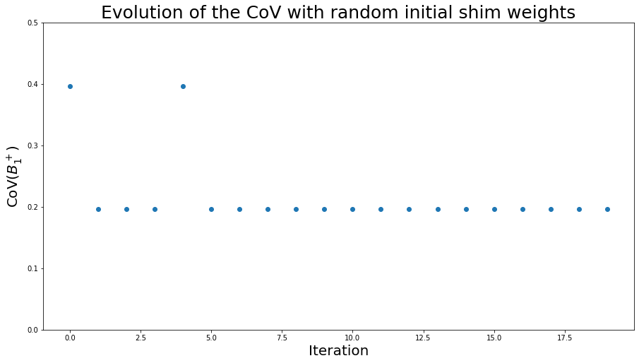
To illustrate the issue of global vs. local minimum during optimization, let’s run phase-only shimming several time with different random initial shim weights, and observe the CoV values:
CoV_vector = []

for _ in range(20):
    # Run the phase-only shimming algorithm with random initial shim weights between 0 and 2pi
    weights_PO = phase_only_shimming(b1_maps, mask, 2*np.pi*np.random.rand(n_Tx))
    b1_PO = np.abs(b1_maps @ weights_PO)
    CoV_vector.append(variation(b1_PO[mask]))

plt.figure(figsize=(15, 8))
plt.plot(CoV_vector, 'o', linewidth=3)
plt.ylim(0, 0.5)
plt.title("Evolution of the CoV with random initial shim weights", fontsize=25)
plt.xlabel("Iteration", fontsize=20)
plt.ylabel("CoV($B_1^+$)", fontsize=20)
plt.show()
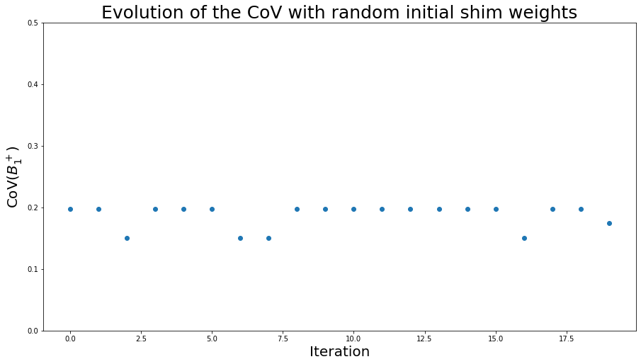
This graph shows different CoVs depending on the initialization parameters for the optimization. Despite this variability, all these CoVs are still lower than when using the CP mode.
With simulated \(B_1^+\) maps
If we reproduce similar phase-only shimming experiments with simulated data, we observe that the phase-only shimming almost always results in the same \(B_1^+\) distribution as the CP mode, further illustrating how optimal the CP mode can be for circular volume coils imaging perfectly circular and homogeneous objects. But again, this is not the case for “real world” in vivo human imaging.
Note
We wrote almost always because in a few cases (approximately 1 time out of 50), the initial weights are very close to a sTx excitation, which is a local minimum, so the optimization converges toward a sTx \(B_1^+\) distribution. A few other local minima exist and result in different \(B_1^+\) distributions. If it is the case on the images below, which are randomly generated, consider yourself unlucky and feel free to run the Jupyter book again!
We can also observe that the phase-only shimmed weights might be phase shifted compared to the CP mode weights, and the polarization direction changes half of the time as both cases results in the same \(B_1^+\) distribution.
b1_maps, _ = simulate_b1_maps(n_Tx, 90)

weights_sTx = np.ones(n_Tx)  # Single pulse weights
b1_sTx = b1_maps @ weights_sTx

weights_CP = np.exp(1j * np.linspace(0, 2*(np.pi - np.pi / n_Tx), n_Tx)) # CP weights
b1_CP = b1_maps @ np.exp(1j * np.linspace(0, 2*(np.pi - np.pi / n_Tx), n_Tx))

mask = b1_maps[:, :, 0] != 0  # 2D mask removing null values

weights_PO = phase_only_shimming(b1_maps, initial_weights=2*np.pi*np.random.rand(n_Tx))

b1_PO = b1_maps @ weights_PO  # Computing the complex phase only shimmed B1+ field

fig, axes = plt.subplots(1, 3, figsize=[20, 7])
vmax= np.max(np.abs(np.concatenate((b1_sTx, b1_CP, b1_PO))))

axes[0].imshow(np.abs(b1_sTx), vmax=vmax); axes[0].axis('off')
axes[0].set_title(f"$|B_1^+|$ (sTx)\nCoV = {variation(np.abs(b1_sTx[mask])):.2f}", fontsize=20)

axes[1].imshow(np.abs(b1_CP), vmax=vmax); axes[1].axis('off')
axes[1].set_title(f"$|B_1^+|$ (CP mode)\nCoV = {variation(np.abs(b1_CP[mask])):.2f}", fontsize=20)

im = axes[2].imshow(np.abs(b1_PO), vmax=vmax); plt.axis('off')
plt.title(f"$|B_1^+|$ (phase-only)\nCoV = {variation(np.abs(b1_PO[mask])):.2f}", fontsize=20)

cbar = fig.colorbar(im, ax=axes.ravel().tolist(), shrink=0.72, pad=0.015)
cbar.ax.set_title('nT/V', fontsize=20, pad=10)
cbar.ax.tick_params(labelsize=20)

plt.show()

plt.figure(figsize=[17, 8])
plt.suptitle("Complex shim weights", fontsize=30, y=1.05)
plt.subplot(131)
show_weights(weights_sTx)
plt.title("sTx", fontsize=30, pad=15)
plt.subplot(132)
show_weights(weights_CP)
plt.title("CP mode", fontsize=30, pad=15)
plt.subplot(133)
show_weights(weights_PO)
plt.title("Phase-only shimming", fontsize=30, pad=15)
plt.show()

CoV_vector = []

for _ in range(20):
    # Run the phase-only shimming algorithm with random initial shim weights between 0 and 2pi
    weights_PO = phase_only_shimming(b1_maps, mask, 2*np.pi*np.random.rand(n_Tx))
    b1_PO = np.abs(b1_maps @ weights_PO)
    CoV_vector.append(variation(b1_PO[mask]))

plt.figure(figsize=(15, 8))
plt.plot(CoV_vector, 'o', linewidth=3)
plt.ylim(0, 0.5)
plt.title("Evolution of the CoV with random initial shim weights", fontsize=25)
plt.xlabel("Iteration", fontsize=20)
plt.ylabel("CoV($B_1^+$)", fontsize=20)
plt.show()